Understanding Transformer Architecture from First Principles: A Detailed Exploration

Introduction

Transformer Architecture lies at the heart of modern AI models. Nearly all the state-of-the-art large language models(LLMs) like ChatGPT, LLaMa and Gemini ,all of them are built upon the transformer architecture.The transformer architecture was introduced in the paper Attention is all you need [^1]. Although it is used everywhere these days,it was first introduced for the purpose of language translation but then it was quickly generalized to other task as well.Since then, due to its scalability and self-attention mechanism it has found itself in not just natural language processing(NLP) but also in computer vision,speech and multimodal AI systems.

In this blog, we will explore the internals of the Transformer Architecture ,with mathematical intuition and understand why it became the backbone of generative AI.

Problems with RNN’s and Sequence models

Before transformers, many natural language processing task were done using sequence models like recurrent neural network(RNN’s).RNNs had major flaws due to which it was not good enough for most language-based applications.Lets discuss their flaws and how transformer massively improved upon them

1) Vanishing/Exploding Gradient problem

One of the major problems with RNNs were the vanishing/exploding gradients.

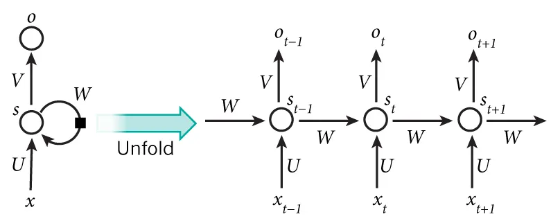
Credit: dennybritz.

The above diagram shows an RNN being unfolded/unrolled across time steps.We essentially have a full network for all the input sequence.For a sequence of 10 words/tokens the network would be unrolled into a 10 layer network one for each time step.This is fine for smaller sequences but for longer input sequences,the network becomes very deep

As a result during, backpropagation through time(BPTT) the gradient at each step would propagate backwards through many steps, this could cause the gradient to be extremely small causing a Vanishing Gradient Problem or the gradient could become very large which would cause the weights to be updated by large amount leading to numerical overflow causing a Exploding Gradient Problem.

2) Handling Long term dependencies

The correct completion is “Nepali” but for the model to correctly predict it. It needs to store the context word “Nepal” which appears 15-20 tokens before the target, diluted by many intermediate states. without the context of “Nepal” the model has no clue to guess the target

3) Sequential Processing

RNN’s rely on sequential processing, meaning the next output at each step depends on the previous step. Mathematically, for seqeunce of $x_1,x_2,x_3,\dots ,x_n$

$$h_t=f(h_{t-1},x_t)$$ where hidden state at time step $t$ depends upon previous step. we cant calculate $h_t$ without calculating $h_{t-1}$ first. Unlike CNNs or Transformers where many computations could occur simultaneously. RNNs cannot make use of parallel computations, they are stuck in a chain-like process.

Because of these limitations it was of no use when it came to handling large seqential data, this makes them slow,ineffective and limited. These problems are completely solved in modern architectures like Transformers

Architecture Overview

Lets look at the Overall architecture of Transformer model and go into each section and dicuss that in detailed later in the blog

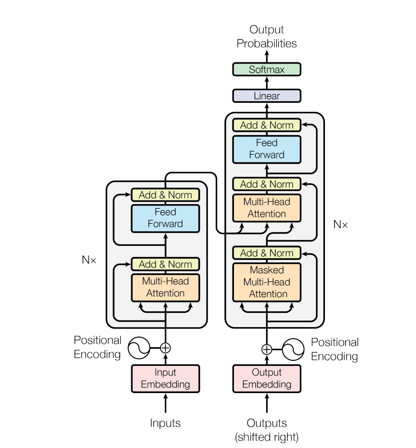
[^1]

Transformer architecture consist of two main components: encoder and a decoder. The encoder takes in an input sequence(tokens) and converts it into numerical vectors that captures its meaning and relationship with each other. The decoder uses these encoded representations along with the tokens it has already generated to provide us with a probabilty distribution of possible next tokens at each time step.

We will get into the details of each and every step later in this blog.

Positional Encoding

Unlike CNNs and RNNs, Transformers which uses self attention is Permutation Invaraint meaning a it doesnt care about what order the tokens came in. It treats them as a bag of vector. For example a input sequence " Ram pushed Hari" and “Hari pushed Ram” would look the same to the transformer without positional information.

To address this we inject position information to the input sequence embeddings before feeding them to the transformer layers.

We want the model to identify which tokens are nearer and which are futher distant. Note: These are not learnable positional encodings rather static

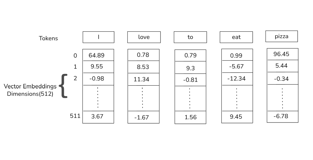
Each input token is first mapped to a vector embedding of dimension 512(in the paper) Credit: Author.

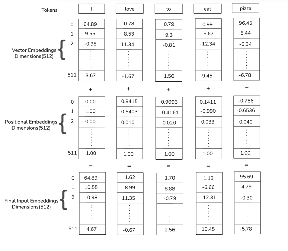
Above figure shows how each input token is mapped to a vector of a fixed dimension but it lacks positional information.Its solution lies in adding another vector positional encoding vector of same dimension(512) to the original vector embedding.

$$E_{final}(pos,token)=E_{word}(token)+PE(pos)$$

Where:

• $E_{word}(token)$ is the 512 dimensional token embedding(as shown in the diagram)
  
• $PE(pos)$ is the positonal encoding vector for position $pos$

To calculate this we have positonal encoding fourmula as: $$PE(pos,2i)=sin(\frac{pos}{{10000}^{\frac{2i}{d_{model}}}})$$

$$PE(pos,2i+1)=cos(\frac{pos}{{10000}^{\frac{2i}{d_{model}}}})$$

Where:

• $pos$ = token position(0,1,2….)
  
• $i$ = dimension index(0 to 255 for 512-dimension embeddings)
  
• $d_{model}$ = embedding dimesion(512)

So odd dimensions(0,2,4,…) takes the cosine fourmula whereas even dimension(1,3,5,..) takes sine fourmula Credit: Author.

Now the question aries on how does adding the positional encodings generated by these trignometric fourmula help the model gain positional information on input sequence.

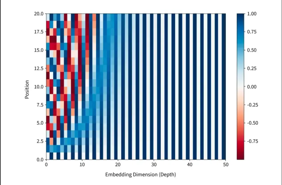
Credit: sercaler.

In the above chart were X-axis represents encoding dimensions and Y-axis represents different position in sequence,a particular cell’s intensity is the sine/cosine value. we can clearly see a visible pattern in this chart the left side High intensity changes creates a checkerboard pattern and on the right side Smooth intensity changescreates a smooth gradients.

Rapid color changes means that model can distinguish between nearby positions and smooth color changes means model understands broad position relationships, with this each position gets a unique fingerprint.

Different frequencies of sine/cosine functions create the intensity variations you see, giving each position a unqiue pattenr across all dimensions

Self-Attention Mechanism

Before going deep towards the mathematics of self-attention lets first look self- attention from a higher level.Self attention lets each token look at every other token in the seqeuence and determine how much each if them matters when building new representations.The “self” in self-attention simply refers to the the fact that it uses the surrounding words within the sequence to provide context.This can all be done in parallel which can leverage parallel processing for faster computations.

Visualising self-attention

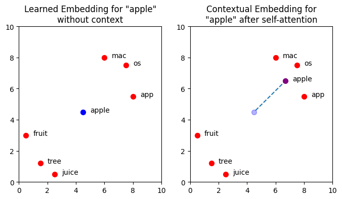
Simply speaking the goal of self attention is to move/change the vector embedding for each token to a embedding vector spcae that better represents the context. For example: we have a word/token “Apple”, now apple has mutilple meanings,it could be the fruit apple or the company apple that makes iphones. Now if we visualize this in a 2-Dimensional vector space it would probably lean more towards the fruit clusters. Now if theres a context say u ask

Now since apple has multiple meanings , since we are talking about the tech company “Apple”.Now the word/token apple must be shifted towards the technological side from the fruits/juices side in the embedding vector space.Below is a 2-Dimensional visualization for this.

import matplotlib.pyplot as plt

# Create word embeddings
xs = [0.5, 1.5, 2.5, 6.0, 7.5, 8.0]
ys = [3.0, 1.2, 0.5, 8.0, 7.5, 5.5]
words = ['fruit', 'tree', 'juice', 'mac', 'os', 'app']
apple = [[4.5, 4.5], [6.7, 6.5]]

# Create figure
fig, ax = plt.subplots(ncols=2, figsize=(8,4))

# Add titles
ax[0].set_title('Learned Embedding for "apple"\nwithout context')
ax[1].set_title('Contextual Embedding for\n"apple" after self-attention')

# Add trace on plot 2 to show the movement of "apple"
ax[1].scatter(apple[0][0], apple[0][1], c='blue', s=50, alpha=0.3)
ax[1].plot([apple[0][0]+0.1, apple[1][0]],
           [apple[0][1]+0.1, apple[1][1]],
           linestyle='dashed',
           zorder=-1)

for i in range(2):
    ax[i].set_xlim(0,10)
    ax[i].set_ylim(0,10)

    # Plot word embeddings
    for (x, y, word) in list(zip(xs, ys, words)):
        ax[i].scatter(x, y, c='red', s=50)
        ax[i].text(x+0.5, y, word)

    # Plot "apple" vector
    x = apple[i][0]
    y = apple[i][1]

    color = 'blue' if i == 0 else 'purple'

    ax[i].text(x+0.5, y, 'apple')
    ax[i].scatter(x, y, c=color, s=50)

plt.show()

Credit: Author.

Mathematical implementation of single head self-attention

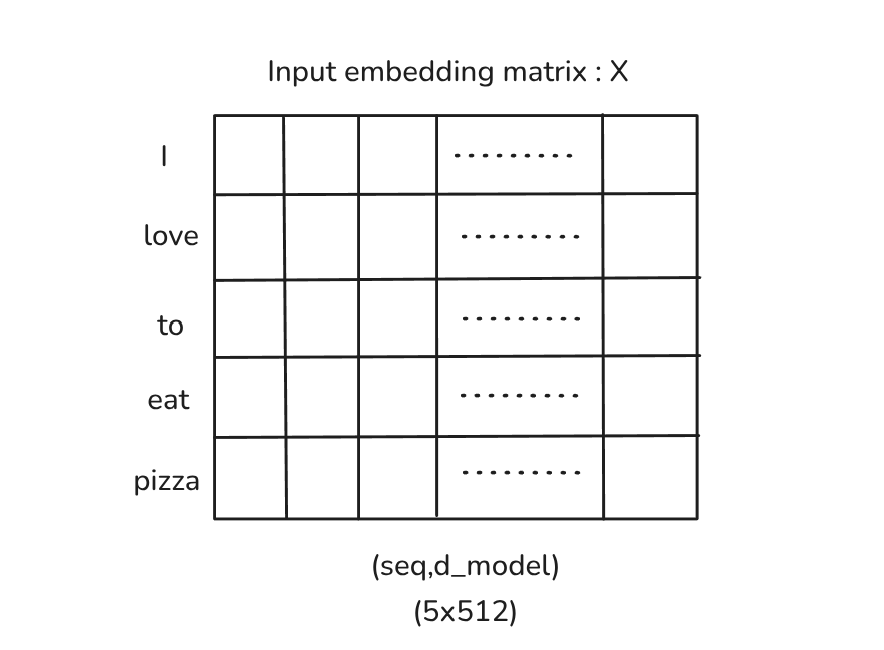
Now, we have seen what self-attention is and how it works at a higher level, we will dive deep into how it is implemented mathematically.In this simple case lets consider the sequence we used earlier

we obtain a input embedding matrix after positional encoding step as such:

Credit: Author.

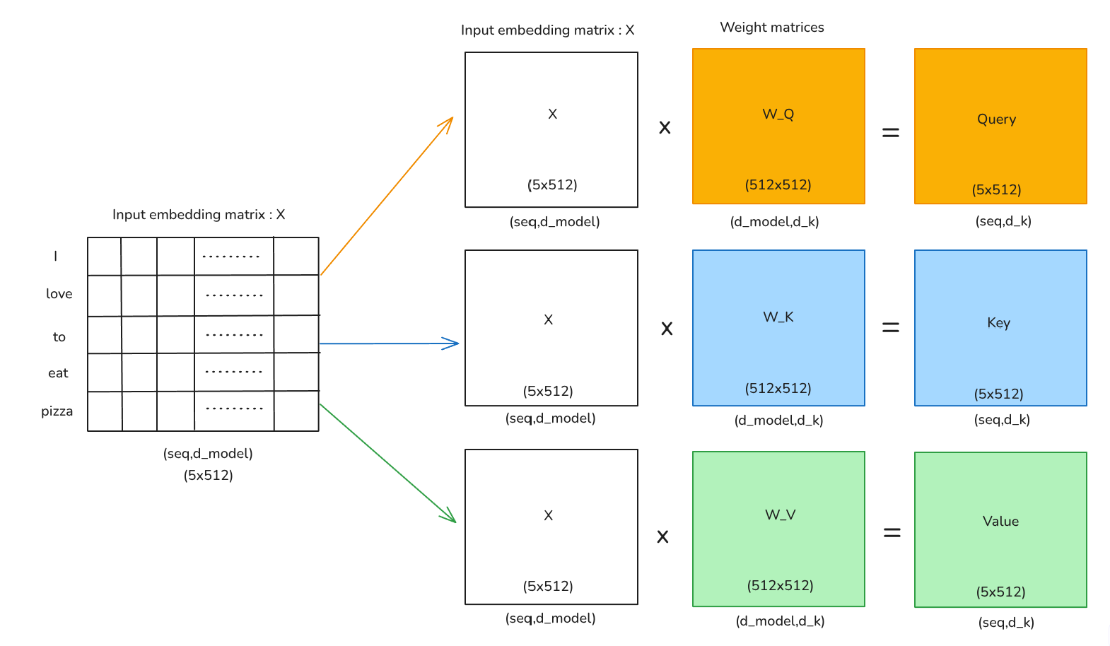
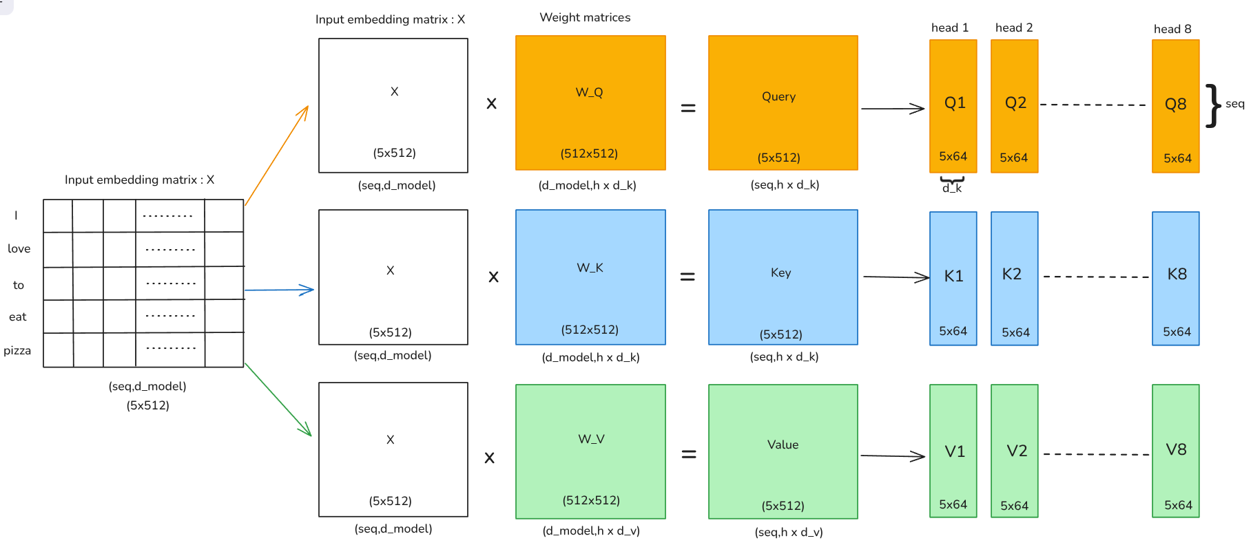
for a single head self attention we have to first project the matrix $X$ into three different matrices,key, query and value. these are linear projections of input embeddings obtain by mutlipy with three different weight matrices $$W_Q\in {\mathbb{R}}^{512\times d_k}$$ $$W_K\in {\mathbb{R}}^{512\times d_k}$$ $$W_V\in {\mathbb{R}}^{512\times d_v}$$

then finally u compute matrices Q,K,V by multiply these learnable weight matrices to the input embedding matrix:

$$Q=X.W_Q$$ $$K=X.W_K$$ $$V=X.W_V$$ then for this case as $X$ is $(5\times 512$) we choose $$d_k=d_v=512$$

Credit: Author.

The obtained Query,Key and Value matrices are now used to calculate the attention score through self-attention fourmula $$Attention(Q,K,V)=softmax(\frac{Q{K}^T}{\sqrt{d_k}})V$$ From this fourmula,before we get attention scores we first calculate similarity scores between tokens using query and key vectors: $$Similarity=Q{K}^T$$ Raw similarity scores can be +ve,-ve , large or small, higher similarity means words.token are more related . These similarity scores are scaled then passed through softmax to normalize all scores to sum to 1.0. It essentially converts raw similarity to probability like weights.

The output after applying this fourmula would be a attention score matrix of size $5\times 5$. where the attention score determine how much each word/token pays attention to every other word including itself.The matrix will look something like this:

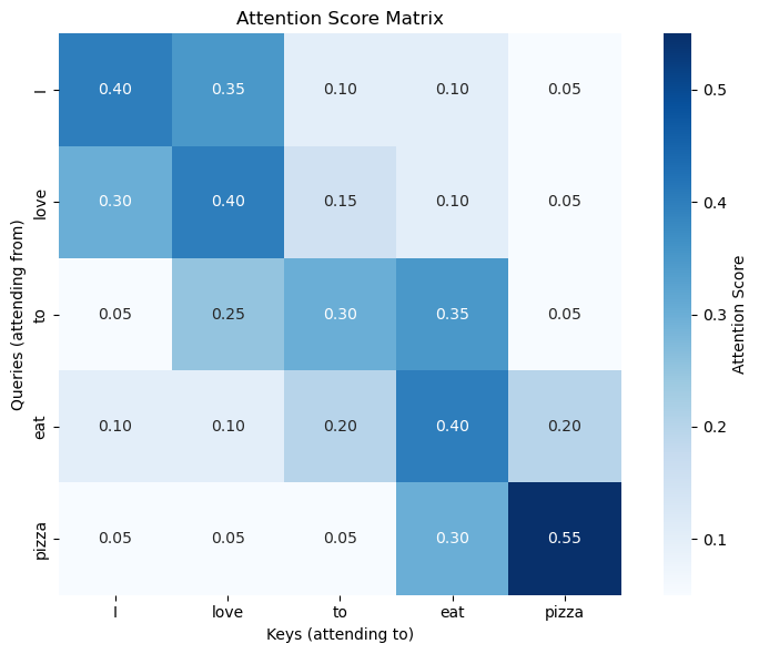
Credit: Author.

Each row become as probability distribution whose sum is 1.0.Each cell shows attention score between two words

What we can observe is that every token pays most attention to itself, as seen in the diagonal. we can also see ‘pizza’ has the strongest self-attention and connects strongly to ’eat’ which shows how model has understood relationships between words, subjects connect to verbs, verbs connect to objects.

Problem with single-head self-attention

Single head works but plateaus in performance as a single head self-attention only limits us to a single view of similarity. Natural language is rich and ambigiuos , a single sentence carries multiple layers of information simultaneously such as

• Syntatic strcuture- which words are subject,verbs,objects,etc
• Semantic relationship - which words relate in meaning(“dog” “barks”)
• Contextual meanings - sentiment(“happy” might mean smile)

A single head cannot capture all these aspect limiting us, so to tackle this problem multi-head attention is used

Multi-Head Attention

Since, we already discuss the problem with single head self-attention lets discuss how multi-head attention mechanism works.

Multi-Head Attention splits the attention mechanims into $H$(H=8 in paper) independent heads, each learning its own smaller set of learnable parameters in parallel and concating them at last.Each head works in a smaller subspace $$d_k=d_v=\frac{d_{model}}{h}=512/8=64$$ dimension of each head becomes 64.The spliting happens in the following fashion

Credit: Author.

$$Q\to [Q^{(1)},Q^{(2)},\dots .,Q^{(8)}],Q^{(i)}\in {\mathbb{R}}^{5\times 64}$$ Similarly for K,V

Self-attention per Head

$$Attention(Q^{(i)},K^{(i)},V^{(i)})=softmax(\frac{Q^{(i)}{K^{(i)}}^T}{\sqrt{64}})V^{(i)}$$

Output of each head: $$H^{(i)}\in {\mathbb{R}}^{5\times 64}$$

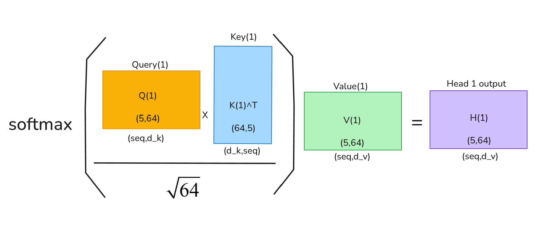
Credit: Author.

At last all output heads are concatenated: $$H=[H^{(1)}|H^{(2)}|\dots ..|H^{(8)}]$$ where $H\in {\mathbb{R}}^{5\times 512}$

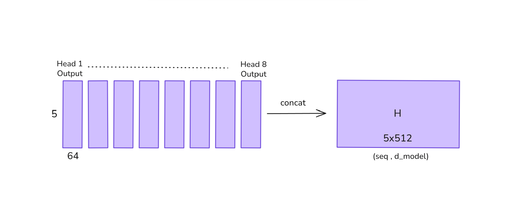
Credit: Author.

Finally a linear projection is applied to bring to the original model dimension: $$Multihead(X)=H{W}_o$$

where: $W_o\in {\mathbb{R}}^{512\times 512}$

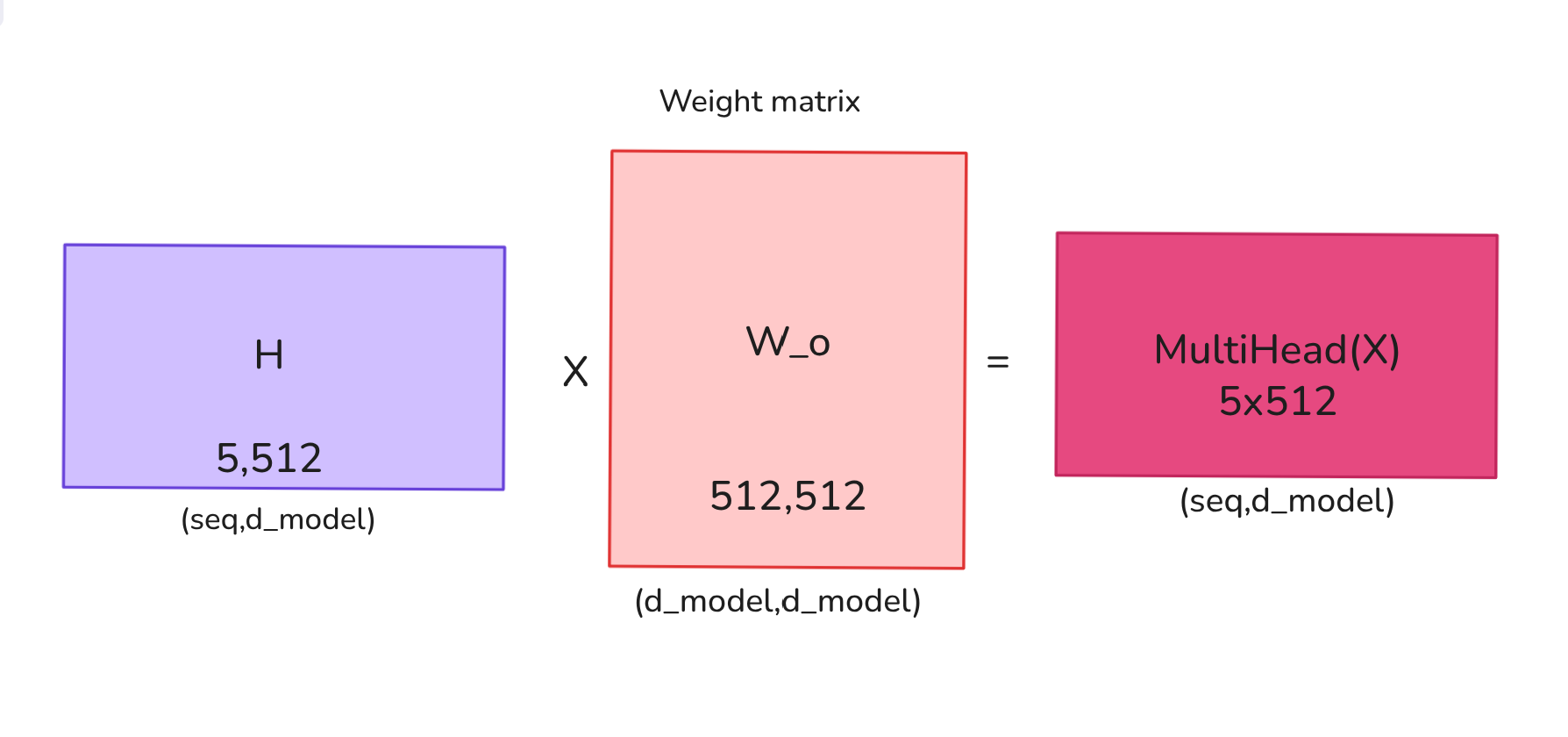
Credit: Author.

Thus, the final output of multi-head attention is obtained. The output dimensions might look the same as single-head self attention but it now carries a deeper more rich representation of input which helps to improve its performance even further.But this isnt the full picture, we still need to look at feed-forward layers,resisdual connection ,layer normalization.

References

• Vaswani, A., Shazeer, N., Parmar, N., Uszkoreit, J., Jones, L., Gomez, A. N., Kaiser, Ł., & Polosukhin, I. (2017). Attention is all you need. In Advances in Neural Information Processing Systems (NeurIPS).

• Smith, B. (2024, February 9). Contextual transformer embeddings using self-attention explained with diagrams and Python code. Towards Data Science. https://towardsdatascience.com/contextual-transformer-embeddings-using-self-attention-explained-with-diagrams-and-python-code-d7a9f0f4d94e/