Understanding why modern machine learning models optimize cross entropy and how KL divergence comes into play.
Introduction
Probability distributions are essential to machine learning. Whether we are building a classifier, language model, or generative model, the objective is the same:
Making the predicted probability distribution as close as possible to the true distribution.
But we can’t just subtract the probabilities and find loss/error so,we ask
How do we measure the difference between two probability distributions?
Two of the most fundamental concepts used for this purpose are:
- Cross Entropy
- Kullback-Leibler (KL) Divergence
Although they appear together, they sightly different.
- Cross Entropy measures how many bits are required to encode data from one distribution using another.
- KL Divergence measures the extra information lost when one distribution approximates another distribution.
Understanding these will make it clear why we use cross entropy loss in most of the classification problems.
Probability Distributions
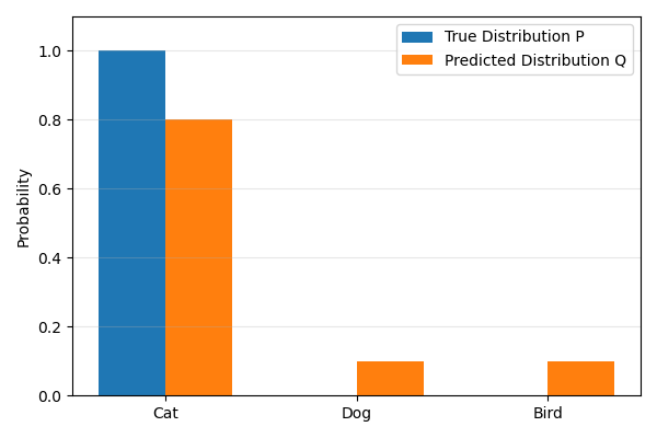
Suppose we have two distributions which shows what we might get during classification problem.
-
True distribution : $P(x)$
-
Predicted distribution: $Q(x)$
Example:
| Class | $P(x)$ | $Q(x)$ |
|---|---|---|
| Cat | 1.0 | 0.8 |
| Dog | 0.0 | 0.1 |
| Bird | 0.0 | 0.1 |
The model predicts:
$$ Q = [0.8, 0.1, 0.1] $$
while reality is
$$ P = [1, 0, 0]. $$
Our end goal is :
$$ Q \approx P. $$
 Credit: Author.
So the question we ask is :
How close are these two distributions? and how do we measure closeness in this scenario
Entropy
Before understanding cross entropy, we first understand entropy.
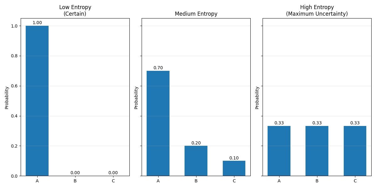
Entropy measures the uncertainty of a probability distribution.
Mathematically,
$$ H(P) = -\sum_x P(x)\log P(x) $$
Intuition
Imagine guessing tomorrow’s weather.
Case 1
If it always rains.
$$ P(rain) = 1 $$
No uncertainty or randomness.
Entropy becomes zero
$$ H(P) = 0 $$
Case 2
Rain and sunshine are equally likely.
$$ P = [0.5, 0.5] $$
Now predicting becomes harder.
Entropy increases or you could say randomness increases
Visually,
 Credit: Author.
Entropy is simply the average amount of information needed to describe outcomes drawn from $P$.
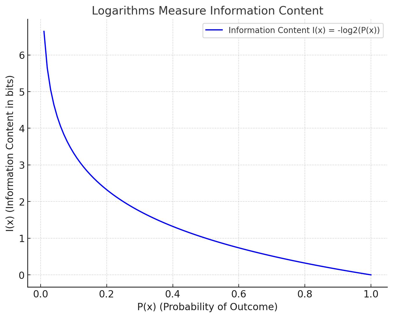
Why the term $-P(x)\log P(x)$?
When we look at the fourmula for cross-entropy is looks unusal, why are we multiplying the probability of event to its logarithm?
The answer lies in the amount of information carried by that event, the event which is very likely doesn’t provide much new information because its certain, but an rare event are more suprising and carry more information.
The expression $-P(x)\log P(x)$ represents the contribution of single outcome to the total entropy.
 Credit: Author.
Cross Entropy
Suppose the true distribution is : $P$
but we encode the data assuming another distribution: $Q$
The average encoding cost becomes
$$ H(P, Q) = -\sum_x P(x)\log Q(x) $$
This is called Cross Entropy.
Important Observation
Notice something interesting.
The true probabilities $P(x)$ are outside the logarithm.
Only $Q(x)$ appears inside the logarithm.
This means:
We average over the true distribution while evaluating the confidence of the predicted distribution.
Example Calculation
Suppose
$$ P = [1, 0] $$
and
$$ Q = [0.8, 0.2]. $$
Cross entropy becomes
$$ H(P, Q) = -(1)\log(0.8) $$
Now,
$$ H(P, Q) \approx 0.223 $$
If instead
$$ Q = [0.99, 0.01] $$
then
$$ H(P, Q) = -\log(0.99) $$
which gives
$$ H(P, Q) \approx 0.010. $$
The loss decreases because predictions become more accurate.
Why Does Cross Entropy Penalize Wrong Predictions?
Consider binary classification problem. Let’s say the correct prediction is Yes/Okay or in binary terms “1”
Correct prediction would be :
$$ Q = 0.99 $$
Calculating Loss:
$$ -\log(0.99) \approx 0.01 $$
Now for wrong prediction:
$$ Q = 0.01 $$
Loss:
$$ -\log(0.01) \approx 4.60 $$
Notice the how sharply the loss increases.The logarithm heavily penalizes confident mistakes, which is what we want from our loss function
KL Divergence
Cross entropy alone does not tell us how much worse our prediction is than the true distribution.
That is where KL Divergence comes in.
It is defined as
$$ D_{KL}(P | Q) = \sum_x P(x)\log \frac{P(x)}{Q(x)} $$
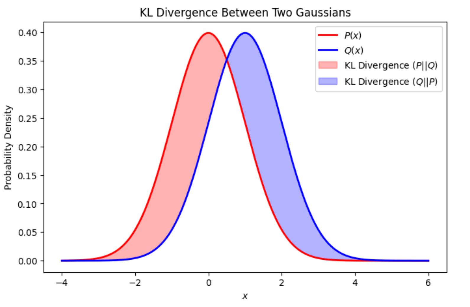
This measures how much information is lost when $Q$ approximates $P$.
Simplified Interpretation
Imagine having:
- the correct map
- an approximate map
KL divergence measures how much additional information is needed because your map is imperfect.
Smaller values mean the approximation is better.
Note : KL Divergence is directional, meaning
$$ D_{KL}(P | Q) \neq D_{KL}(Q | P) $$
 Credit: Author.
Relationship Between Entropy and Cross Entropy
Expanding KL divergence:
$$ D_{KL}(P | Q) = \sum_x P(x)\log \frac{P(x)}{Q(x)} $$
Using product rule of logarithms,
$$ \log \frac{a}{b} = \log a - \log b, $$
we obtain
$$ D_{KL}(P | Q) = \sum_x P(x)\log P(x) - \sum_x P(x)\log Q(x) $$
Recognizing the entropy terms,
$$ D_{KL}(P | Q) = H(P, Q) - H(P) $$
Therefore,
$$ H(P, Q) = H(P) + D_{KL}(P | Q) $$
This is one of the most important identities in information theory.
Why Deep Learning Uses Cross Entropy
During supervised learning, the dataset with labels is fixed.
Therefore,
$$ H(P) $$
is constant.
So,
$$ H(P, Q) = H(P) + D_{KL}(P | Q), $$
So ,minimizing cross entropy is equivalent to minimizing KL divergence because the entropy term is constant.
Mathematically,
$$ \arg\min_Q H(P, Q) = \arg\min_Q D_{KL}(P | Q). $$
Thus, optimizing cross entropy help push the predicted distribution closer to the true distribution.
One-Hot Labels
In classification, labels are usually one-hot encoded. O for No and 1 for Yes.
Example:
True class:
$$ P = [0, 1, 0] $$
Prediction:
$$ Q = [0.2, 0.7, 0.1] $$
Cross entropy becomes
$$ -\left( 0\log 0.2 + 1\log 0.7 + 0\log 0.1 \right) $$
Only the correct class remains:
$$ -\log 0.7 $$
This explains why cross entropy loss for classification is commonly written as
$$ L = -\log(p_{\text{correct}}) $$
where $p_{\text{correct}}$ is the predicted probability assigned to the true class.
Geometric Interpretation
Imagine every probability distribution as a point in a high-dimensional space.
- Entropy describes the uncertainty of one point.
- Cross entropy measures how well one point explains another.
- KL divergence measures the gap between them.
As training progresses, the predicted distribution
$$ Q $$
moves closer to
$$ P. $$
Eventually,
$$ Q = P $$
and
$$ D_{KL}(P | Q) = 0. $$
At this point,
$$ H(P, Q) = H(P), $$
meaning there is no additional information cost from using the predicted distribution.
Conclusion
Entropy, cross entropy, and KL divergence are fundamental to machine learning optimization.
- Entropy measures uncertainty within a distribution.
- Cross entropy measures how well a predicted distribution models the true one.
- KL divergence quantifies the additional information lost due to approximation.
They relate by,
$$ H(P, Q) = H(P) + D_{KL}(P | Q), $$
This explains why minimizing cross entropy is same as minimizing the KL divergence when true distribution $P$ is constant, this help explain the principles of training neural networks, language models and countless other probabilistic models.
Ultimately, improvement in model’s prediction can be seen as reducing the information gap between what model believes $Q$ and how world actually behaves $P$